Quantifying Diversity - many metrics, in
three dimensions
Here is some advice (inspired by the
ideas presented on this website) for those who want to measure the
biodiversity of a system in practice. (written by Keith Farnsworth).
You might like to first examine my introductory lecture slides on biodiversity here, and the slightly more advanced presentation (given to an Imperial College, London audience in 2018) here.
(the diagrams on this page are taken from it)
You might like to first examine my introductory lecture slides on biodiversity here, and the slightly more advanced presentation (given to an Imperial College, London audience in 2018) here.
(the diagrams on this page are taken from it)
Overall concept
The general
idea is that a biological system is composed of a set of N components which can be
categorised (partitioned) into S
component-types which differ from one another in a quantifiable way. Each type (take
the i'th type) accounts for a
proportion p_i of the total N.
That would be enough if we are describing the diversity of a mere
sample of components (e.g. species in a quadrat), but underlying this,
we usually want to imply the biodiversity of the system as a whole
(especially an ecological community), so we should also include the
diversity of interactions among the components. This is a separate and
rather neglected issue, which I will deal with further down the page.
For now, consider the sample in diagram 1.It is important to realise
that its diversity is that of a mere sample, not the system from which
it was drawn.
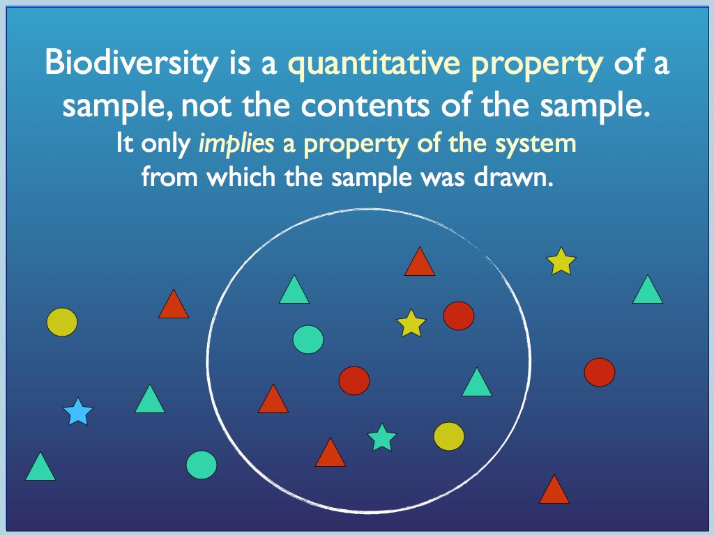
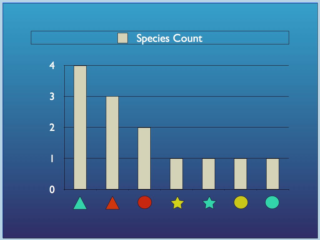
Diagram 1 a) components identified
by
traits (colour and shape) may be categorised in different ways, by
trait or by species (a combination of traits); b) all so called
'structural' biodiversityindices are summaries of the
category-frequency distribution (the p_i
referred to above).
We can make an almost unlimited set of
biodiversity indices out of the frequency distribution of components
among their classes. We also have a choice of classification schemes:
by taxonomic unit (species, family, order, etc..); by traits (such as
dentition in mammals or flower type in flowering plants); by genotypic
metrics (notably using the gene-based phylogeny) or by functions (e.g.
guilds of different organisms such as trophic levels). This
choice can be organised (to some extent) by considering it in terms of
a) the order (i.e. scale) of organisation (e.g. species vs. family) and
b) the character concept (i.e. genetic, function, or taxonomic unit).
It is important to realise that all the possible indices are just that
- they are not biodiversity in and of themselves, they only indicate it
(sometimes very indirectly). I hope it goes without saying that
biodiversity is explicitly not the organisms contained in a system - it
is a measure of the degree of difference to be found in the system and
only that. Notice too that the concept appliesto all levels of
organisation from assemblies of molecules all the way up to the global
ecosystem.
Biodiversity Indices
There are many traditional indices attempting to summarise the distribution of Diagram 1b (e.g. species richness, Simpson's index, Shannon-Weiner index, Jaccard index, Rao quadratic entropy and so on...). They are landmarks in the historical development of the field and all have unique properties, some desirable, some not; people have their favourites, or make more or less rational decisions about which to use, but no single index can ever represent all the information of the distribution. Like statistical moments (mean, variance, skew, etc.) they could be thought of as summaries emphasising different properties of the distribution. Except that they are not like statistical moments in that they are not independent of one another and do not form an ordered set: many are closely related and some have quite bizarre properties.
Dissatisfied with all this, but inspired by the idea of statistical moments, Mark Oliver Hill came up with a way to build indices from a generating function: a general form with a single parameter that when varied creates a set of related indices. When applied to a sample, the resulting metrics are now termed “Hill numbers” and also "effective number" indices.
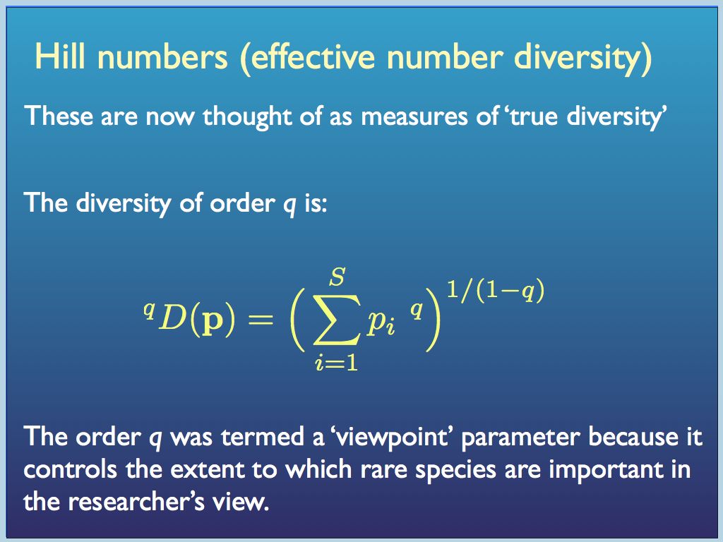
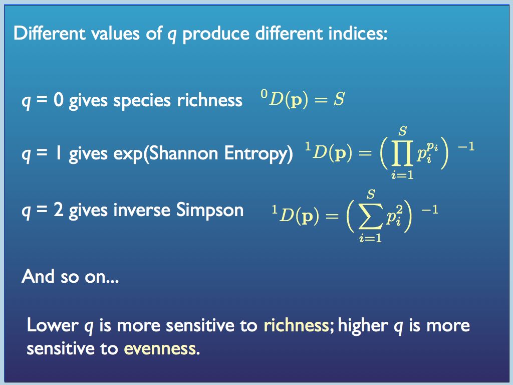
In this generating function p is the vector of proportions {p_1, p_2, ... p_i ... p_S} and q was initially thought of as an integer, but it does not need to be.
Hill number diversity indices have more intuitive properties than traditional indices. In particular, for any set of equally distributed (p_i = p_j for all i,j) components, if the number N is doubled, then all the diversity indices double too. That is certainly not the case for traditional indices (e.g. the Simpson's index actually halves when N is doubled!). Every Hill number (order q) is the diversity of an equivalent sample in which components are equally distributed. For this reason, Hill number values are referred to as equivalent numbers. The great merits of Hill's system are promoted by Lou Jost at his website here. He and also Anne Chow are leading advocates of the approach and have helped to organise, apply and promote it.
There remains at least one problem, though. You will notice that so far we have only shown how to account for the distribution among abundances of components (counting them) and said nothing about the degree of difference among them.
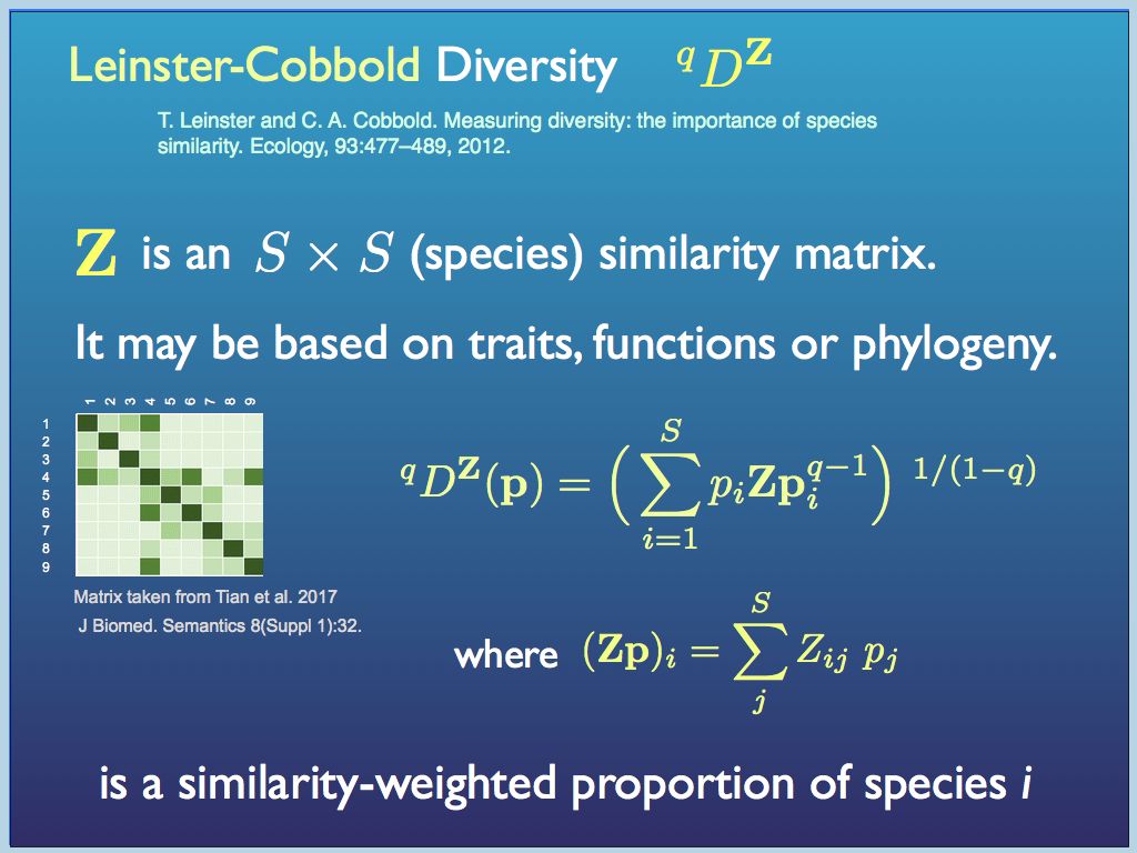
Degree of difference can be quantified in several respects, but one of the most important in biodiversity is phylogenetic (i.e. the evolutionary distance among species). All degree of differences are found from the distances, in some metric, between pairs of component. This is the same as the trianular table of distances between cities that you can find in some old atlases or road maps (if you remember them). For biodiversity, the distance metric is a measure of the number of individual genetic differences, often represented by the number of branch levels you have to traverse in the evolutionary tree (perhaps scaled by genetic clock time if the data is available). At the root of it is the number of mutations in the genome of any pair of organisms. Just like the distance table in an old atlas, the distances (e.g. A-B; A-C; B-C....) can easily be arranged in a 'distance matrix', or equivalently a 'similarity matrix'. By incorporating one of these into Hill's diversity index generating function, Mark Leinster and Christine Cobbold enabled both the count information and the degree of difference among the components to be quantified simultaneously. At present, the Leinster-Cobbold Diversity (with a continuously varying q) is about the last word in quantifying the diversity among components of a sample (see a preprint of their paper here for details). Essentially the innovation is to replace the p_i terms with a similarity (or difference) weighted proportion of each species. The similarity weighting used for each species i is the average pairwise similarity between between the ith species and every other species (this is explained in the dispay below.
Biodiversity Dimensionality
So far we have considered two kinds of diversity - the distribution of numbers of things in a sample and the degree of differences among the things. The mainstream interpretation of these in biodiversity is that they represent the biological complexity of the system from which a sample is taken. Followers of this website will say it represents the information content of the sample and by implication, of the system. Broadly speaking, biodiversity arises from genetic variation (the reason for e.g. species differences), ecological structure (the network of interactions and population abundances) and the diversity of functions performed by system components (e.g. nitrogen fixing). Knowing that gives us a more concrete understanding of biodiversity. Diversity is differnece and the differences among organims, their distribution and their functional relationships are all embodied in the living ecosystem and all contribute to total biodiversity.
Together, these aspects form three major axes of biodiversity (see Lyashevska & Farnsworth 2012): implying that biodiversity is effectively three-dimensional. Of course that is a kind of simplification used to make the problem of quantification more tractable, but the concept behind it also helps to understand biodiversity as a source of ecological function. Clearly it is the functional diversity that directly relates to function, but this kind of diversity would be impossible without the components (phylogenetic variation) and structure (structural diversity) underlying it. The reason functional diversity is empirically (more or less) independent of the other two is that there are very many ways of combining phylogenetic and structural elements to produce a set of functions. Again we find embodied information lying behind the diversity of function.
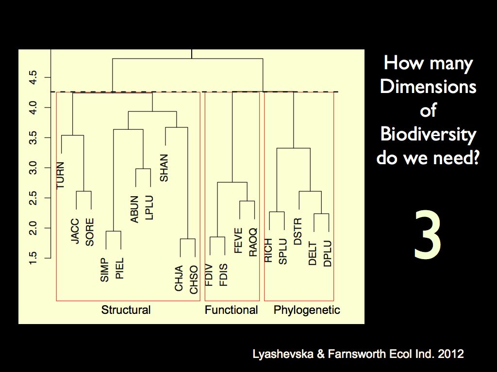
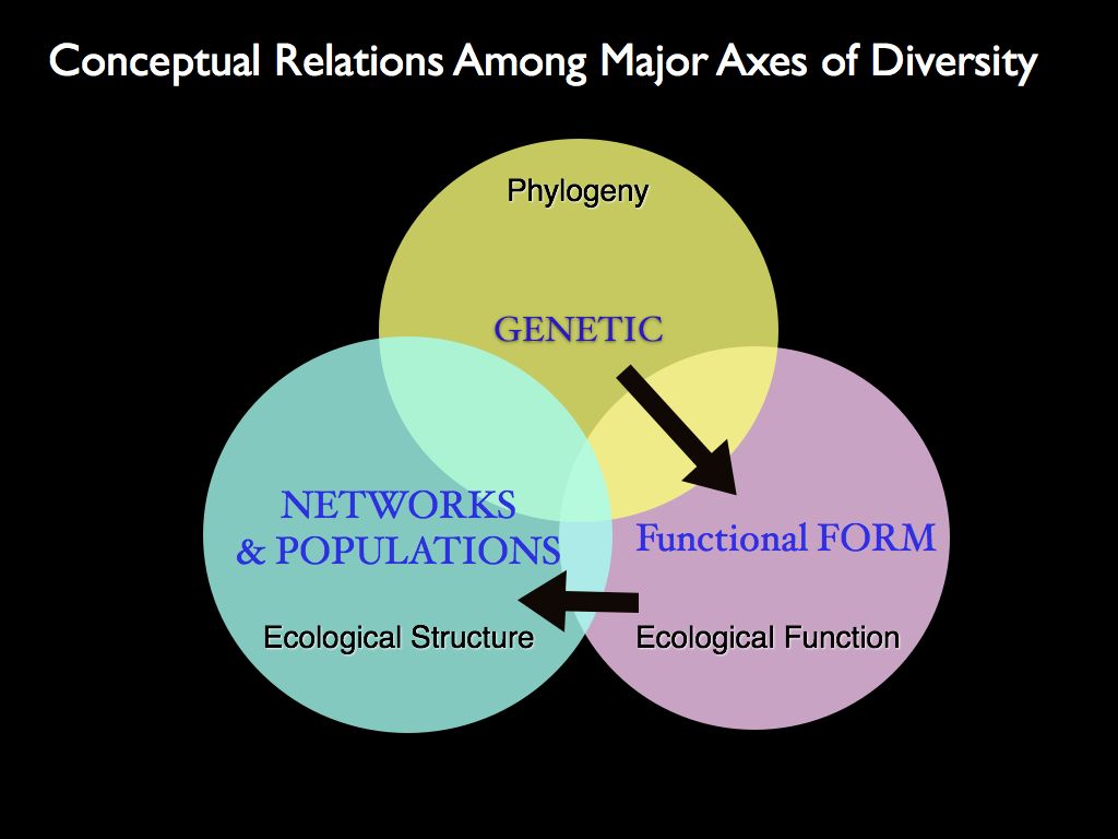
The left panel shows a cluster analysis of different biodiversity
metrics. It demonstrates the
relative relatedness of biodiversity metrics in each of the three
conceptual characters: 'structural', 'functional' and 'phylogenetic'.
It shows that different metrics calculated on a given character are
much more similar than the same metric calculated on a different
character. This is the basis on which we say that there are three
distinct 'major axes' of biodiversity. The right panel shows the
conceptual relationships between the characters: genes inform form,
form specifies function and functions combine (and are selected for) at
the community structure level.
Including system structure
So far, 'structure' has been vaguely regarded as something to do with the relative numbers of different parts in the sameple (the distribution of p_i). A moment's thought about engineered or natural structures in real life reveals that is not structure in any useful sense.
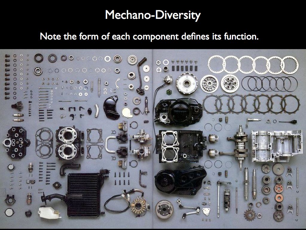

Imagine describing the structure of the engine on the right by counting the number of different components (as on the left), from which we may calculate various mechano-diversity indices. It is clear that what ecologists have grown accustomed to calling 'structural diversity' has little to do with structure. What makes the engine an engine is the precise spatial relationship every component has with all the others, given that they each have a form that dictates a very specific function. The structure is the precise arrangement of functional forms in relation to one another.
Unfortunately we do not have a method for calculating this meaningful sort of structure in ecosystesms. To do so is one of the aims of the work presented on this website.
There are many traditional indices attempting to summarise the distribution of Diagram 1b (e.g. species richness, Simpson's index, Shannon-Weiner index, Jaccard index, Rao quadratic entropy and so on...). They are landmarks in the historical development of the field and all have unique properties, some desirable, some not; people have their favourites, or make more or less rational decisions about which to use, but no single index can ever represent all the information of the distribution. Like statistical moments (mean, variance, skew, etc.) they could be thought of as summaries emphasising different properties of the distribution. Except that they are not like statistical moments in that they are not independent of one another and do not form an ordered set: many are closely related and some have quite bizarre properties.
Dissatisfied with all this, but inspired by the idea of statistical moments, Mark Oliver Hill came up with a way to build indices from a generating function: a general form with a single parameter that when varied creates a set of related indices. When applied to a sample, the resulting metrics are now termed “Hill numbers” and also "effective number" indices.


In this generating function p is the vector of proportions {p_1, p_2, ... p_i ... p_S} and q was initially thought of as an integer, but it does not need to be.
Hill number diversity indices have more intuitive properties than traditional indices. In particular, for any set of equally distributed (p_i = p_j for all i,j) components, if the number N is doubled, then all the diversity indices double too. That is certainly not the case for traditional indices (e.g. the Simpson's index actually halves when N is doubled!). Every Hill number (order q) is the diversity of an equivalent sample in which components are equally distributed. For this reason, Hill number values are referred to as equivalent numbers. The great merits of Hill's system are promoted by Lou Jost at his website here. He and also Anne Chow are leading advocates of the approach and have helped to organise, apply and promote it.
There remains at least one problem, though. You will notice that so far we have only shown how to account for the distribution among abundances of components (counting them) and said nothing about the degree of difference among them.
Degree of difference can be quantified in several respects, but one of the most important in biodiversity is phylogenetic (i.e. the evolutionary distance among species). All degree of differences are found from the distances, in some metric, between pairs of component. This is the same as the trianular table of distances between cities that you can find in some old atlases or road maps (if you remember them). For biodiversity, the distance metric is a measure of the number of individual genetic differences, often represented by the number of branch levels you have to traverse in the evolutionary tree (perhaps scaled by genetic clock time if the data is available). At the root of it is the number of mutations in the genome of any pair of organisms. Just like the distance table in an old atlas, the distances (e.g. A-B; A-C; B-C....) can easily be arranged in a 'distance matrix', or equivalently a 'similarity matrix'. By incorporating one of these into Hill's diversity index generating function, Mark Leinster and Christine Cobbold enabled both the count information and the degree of difference among the components to be quantified simultaneously. At present, the Leinster-Cobbold Diversity (with a continuously varying q) is about the last word in quantifying the diversity among components of a sample (see a preprint of their paper here for details). Essentially the innovation is to replace the p_i terms with a similarity (or difference) weighted proportion of each species. The similarity weighting used for each species i is the average pairwise similarity between between the ith species and every other species (this is explained in the dispay below.

Leinster-Cobbold Diversity weights the
proportion of each species by its average similarity (or difference)
between it and all other species present and does this within a Hill
number framework, to generate a continuous system of diversity indices,
which taken all together, would fully describe the diversity of any
sample (as an assembly).
Biodiversity Dimensionality
So far we have considered two kinds of diversity - the distribution of numbers of things in a sample and the degree of differences among the things. The mainstream interpretation of these in biodiversity is that they represent the biological complexity of the system from which a sample is taken. Followers of this website will say it represents the information content of the sample and by implication, of the system. Broadly speaking, biodiversity arises from genetic variation (the reason for e.g. species differences), ecological structure (the network of interactions and population abundances) and the diversity of functions performed by system components (e.g. nitrogen fixing). Knowing that gives us a more concrete understanding of biodiversity. Diversity is differnece and the differences among organims, their distribution and their functional relationships are all embodied in the living ecosystem and all contribute to total biodiversity.
Together, these aspects form three major axes of biodiversity (see Lyashevska & Farnsworth 2012): implying that biodiversity is effectively three-dimensional. Of course that is a kind of simplification used to make the problem of quantification more tractable, but the concept behind it also helps to understand biodiversity as a source of ecological function. Clearly it is the functional diversity that directly relates to function, but this kind of diversity would be impossible without the components (phylogenetic variation) and structure (structural diversity) underlying it. The reason functional diversity is empirically (more or less) independent of the other two is that there are very many ways of combining phylogenetic and structural elements to produce a set of functions. Again we find embodied information lying behind the diversity of function.


Including system structure
So far, 'structure' has been vaguely regarded as something to do with the relative numbers of different parts in the sameple (the distribution of p_i). A moment's thought about engineered or natural structures in real life reveals that is not structure in any useful sense.


Imagine describing the structure of the engine on the right by counting the number of different components (as on the left), from which we may calculate various mechano-diversity indices. It is clear that what ecologists have grown accustomed to calling 'structural diversity' has little to do with structure. What makes the engine an engine is the precise spatial relationship every component has with all the others, given that they each have a form that dictates a very specific function. The structure is the precise arrangement of functional forms in relation to one another.
Unfortunately we do not have a method for calculating this meaningful sort of structure in ecosystesms. To do so is one of the aims of the work presented on this website.
The Theme is led by Keith Farnsworth
