

Entropy
Note - I am fairly satisfied with this page now (Feb. 2019) - Keith Farnsworth
Introduction to a strangely difficult, but easy concept
For many, entropy seems to be one of those ideas that behaves like a tomato seed on the plate which you just cannot pick up because it squishes away from fork and knife. One reason for difficulty among experts is the confusion between the thermodynamic definition and that of information theory (we will put that aside until the next section). The vast majority of explanations of information entropy rely on communications theory, but I will not start there. Instead, I am going to start with a very intuitive explanation so you can have a meaningful grasp of the idea and not get lost in numbers.
Many people will already have the idea (a slogan really) that "entropy is the disorder of a system". Please forget that: such mis-explanation is another reason for the confusion.
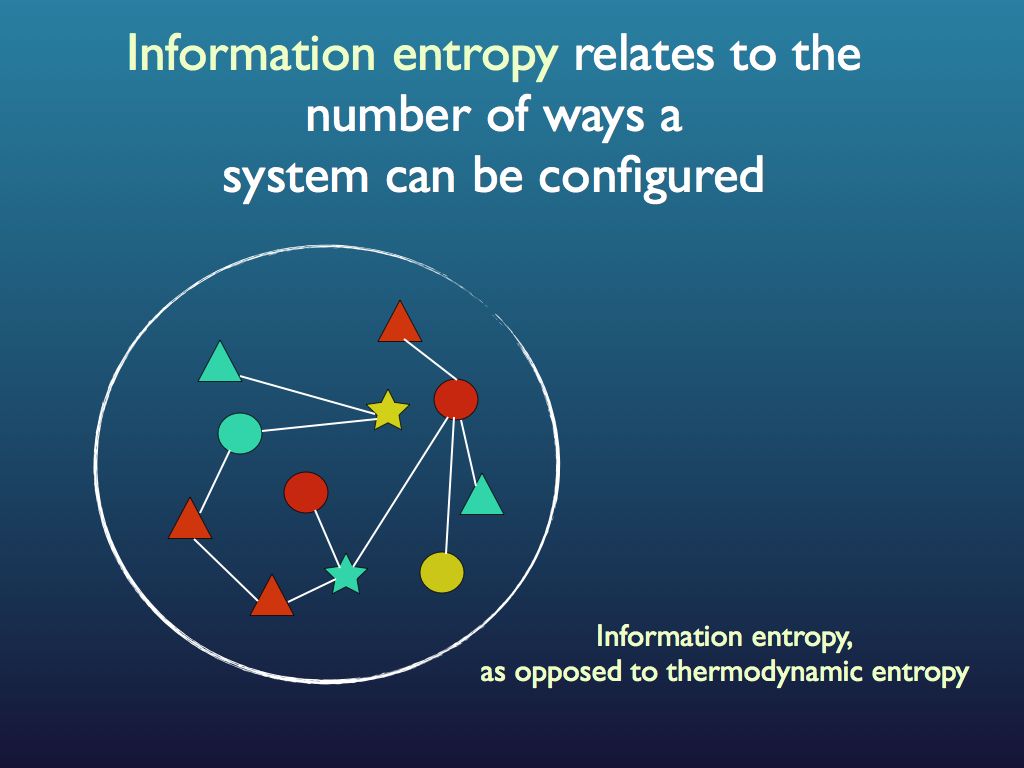
Just to clarify: for the present purpose, we will consider information entropy alone (later, the connection with thermodynamic entropy will be explained). I usually shorten 'information entropy' to 'intropy', by the way.
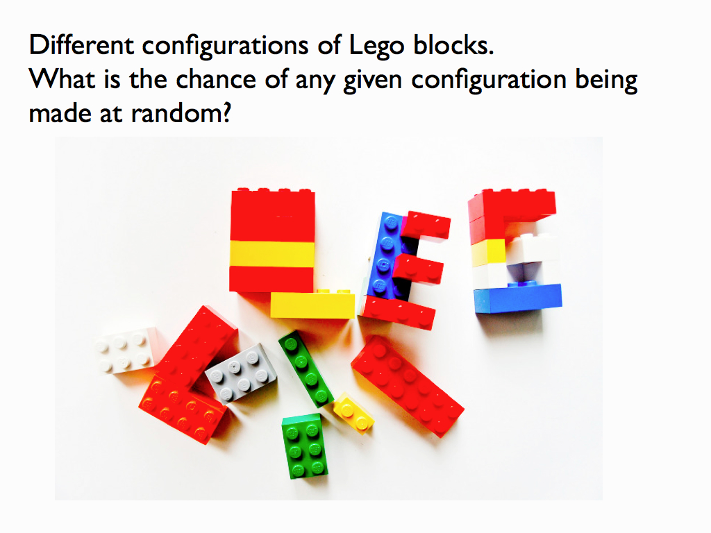
Here is a simple intuitive explanation of entropy that does not rely on communications theory. First, entropy is not a mysterious ‘thing’ (e.g. like energy), instead, it is just a measure of a property that has to do with information. A property of what?, you may ask; the answer is any assembly of objects such as fruit in a fruit bowl, cars in the car park, letters in the scrabble box, molecules in the cytoplasm… As for the property of the assembly that entropy is a measure of: that’s just how many different ways you can arrange the objects in the assembly (see my lego example below). Well, that’s it: entropy is a scientific measure related to the number ways you can arrange things (you see it’s not disorganisation).
The connection with information is just this: if you were to fully describe any particular arrangement of things that you see (so someone could copy it), then you would be giving them information. Intuitively (and in quantitative fact), the amount of information you would need to fully describe the particular arrangement increases as the number of ways it could be arranged increases. For example if there were just three fruits in the bowl and they were all pears, then it would take very little information as the number of ways you could arrange 3 pears is obviously quite small and, sure enough, the entropy of that assembly is very small. If you had an orange, a pear and an apple it would be a bit bigger because you could put different fruit in different orders. If there were 12 fruits, it would be bigger still and by the time you are looking at the molecules in the cytoplasm of an E. coli cell, the amount of information you would need is enormous and so is the entropy. So you see that as the information needed to describe an assembly increases, so does the entropy. Indeed, we can turn this around and see the assembly as a device for holding information, which you can 'read'. The amount of information an assembly can 'embody' in this sense is exactly the same as the amount you would need to describe any particular (one) assembly from among all possible and this increases with the number of ways it can be arranged, which is measured by its entropy. So entropy is also a measure of the amount of information you can pack into an assembly as though that assembly were a code (for example you may have a secret code for your husband that reads: pear, orange, apple in a line = walk the dog / apple, pear, orange = your dinner's in the oven (etc.). I think you can see how many secret messages you can code in the fruit bowl. (If this play leaves you cold, consider instead the signal sequence at the end of a newly secreted protein - it targets the protein to the appropriate location within the cell, rather like a postal (zip) code).
Lastly in this intuitive introduction, I should just mention 'disorganisation'. This notion arises from thinking that an assembly which is arranged as a strong pattern is organised and one in which no pattern is discernible is disorganised (and of course there are a lot more of those). Many explanations of entropy involve an assembly in a box which is partitioned ( e.g. dividing left from right) by an 'imaginary line'. Low entropy systems are those where all of one kind of object are in one side and all of the other are in the other side (pears to the left, apples to the right). This arrangement is just one of several, but if that was your starting point and you were only allowed to rearrange among the fruit in each imaginary compartment (not swapping between them) then clearly that arrangement would be both recognisably organised and low in entropy. The partition idea is really very artificial though and we know that this organised looking assembly is just one of all possible (given freedom to move fruit from one side to the other), so the entropy of the system as a whole is really much higher. Indeed, it does not make sense to talk of the entropy of one particular arrangement, because the point of entropy is: how many possible arrangements is this one an example of. What really made the entropy of the 'organised' assembly seem low was that in this partition-based explanation, there is a hidden assumption that the assembly is constrained to be in that organised configuration. Basically, it says that if all the pears have to stay on the left and all the apples stay on the right (and you cannot tell one pear from another, nor one apple from another), then there is really no way to rearrange this lot and so its entropy is minimised. (The reason I think this explanation abounds is that in developing the idea of thermodynamic entropy, physicists use the partition concept on assemblies of molecules (as in a gas) and end up with the genuinely constrained assembly of a crystal lattice as the lowest thermodynamic entropy arrangement. We are not doing that here).
In a way, that’s it, but to deeply understand this and particularly its implications and the way it enables us to work quantitatively with information embodied in structures, we need to do quite a bit more work (and some of it mathematical). Why do we want to do that? Because working with information embodied in structures is precisely what life does: it stores information in molecular and composite structures and it manipulates that information (computes) by changing those structures. What it computes is itself.
A bit more detailed
So here is the next level of explanation. It uses blocks. It might look a bit complicated until you read it - then you will see it is easy, really.
Suppose you just had three blocks in total, A, B and C. Using the dash "-" to indicate joining blocks together, they can be configured as:
A B C
A-B C
A B-C, or A-B-C. That is just four ways.
So If I made one configuration behind your back and you had to guess which one, the chance of you getting it on first guess is 1/number of possibilities = 1/4. Now if you had to guess which one, using the 20-questions simulation of information (see here), I hope you can see it requires exactly 2 questions to identify the configuration (e.g. "is it in two lumps?" -"it is", then, "is A joined to B?" -"no",
so the configuration is A B-C).
Now let's add another block: D.
The possible configurations are now:
A B C D A-B C-D
A-B C D A-B-C D
A B-C D A B-C-D
A B C-D A-B-C-D,
so changing from 3 to 4 blocks increased the number of configurations from 4 to 8. Given we have 8 configurations, using these 4 blocks, the probability of you correctly guessing which random one I made would be 1/8. Also you would now need 3 binary-answer questions to identify it from quizzing me (see if you can work out a strategy for that). 3 questions for 4 blocks and we had 2 questions for 3 blocks before, in general we need N-1 questions for N blocks.
Notice that the difference among these configurations is all about how many and where the joins (-) appear. For N blocks there are always N-1 possible join sites (this turns out to be the key).
Take a look at the set for N=5. There are 16 possible configurations here:
A-B C D E A-B C D-E A-B-C-D E A B C D E ¤ °
A B-C D E A B-C D-E A-B-C D-E A-B-C-D-E
A B C-D E A-B-C D E A B-C-D-E
A B C D-E A B-C-D E A-B C-D-E
A B C-D-E
A-B C-D E
Now you probably see two patterns emerging. There is the numerical one: every time we add another block we get twice as many configurations. If we call the number of configurations K, then K=2^(N-1).
The other pattern has to do with the joins. Ignore the blocks and just look at the gaps between them (the join sites). We can record the presence of a join in a gap with value 1 and absence of a join with value 0. Then e.g. A-B C D-E is recorded as 1001. This is a binary number of 4 digits, the same number of digits as N-1, the number of join sites (of course). Now we should also know that a binary number of N-1 digits can record any integer number from 0 to (2^(N-1))-1, or more generally, it can record 2^(N-1) different things: we could say that is its information capacity. What we are doing here is making a binary code to represent the configuration and our code can record exactly as many configurations as needed: i.e. 2^(N-1) of them. Remember, the probability of picking one configuration at random (guessing) if there are N blocks is 1/K [this =2^(1-N)] and the number of questions needed to identify it is N-1.
Denoting the number of questions needed as Q, we can easily work K and Q out for any N:
N: 1 2 3 4 5 6 7 8
K: 1 2 4 8 16 32 64 128
Q: 0* 1 2 3 4 5 6 7
* If there is only one block, you know already that there is only one possible configuration, so no questions needed.
The number of questions needed (Q) is the same as the length of the binary code needed to represent all the possible configurations (= the number of join sites = N-1) and so is also the information capacity of the assembly of N elements. You could literally send messages to someone by putting your blocks in particular configurations and the number of different signals you could send would be K (is this a trade secret of Danish spies?).
So now I come to my point about information entropy (intropy). It is a measure of the number of possible configurations we can get out of an assembly of elements (e.g. blocks).
But it is not an arbitrary measure - it has a purpose, otherwise we might as well just use K. The original purpose of intropy was to quantify information. We have just seen that the information capacity of a binary number with length N-1 is K and this is also the information capacity of an assembly of N elements.
One lump or two?
Now suppose you had two separate piles of N blocks each. How many Danish spy signals could you send to your field agent? The answer is not 2K. This is because the two piles when read together amount to an assembly of 2N blocks, for which the number of configurations is 2^(2N-1). [OK, I cheat a little because I am allowing configurations to join blocks across the piles - that is only to keep the maths simple].
Doubling the number of blocks by having 2 piles of N has increased the number of configurations by a lot (something like squared it), but actually it is a bit hard to see. In this situation (working with raised powers of numbers) it is easier to take logs of the whole thing (so powers become multiplications and multiplications become additions). Given we always see 2 raised to a power here, it makes most sense to take logs to the base 2.
Here is how easy it is: log2 (2^(2N-1)) is just 2N-1. We will make a mental note of how helpful log2 transformation could be. Recall that the probability of picking the correct configuration at random (guessing it) is 1/K which for the two piles together, is 1/(2^(2N-1)) = 2^(1-2N) ( log2 transformed, this is just 1-2N, which I hope you can see is a negative number as long as N is not the trivial zero). We will give this probability the symbol p and say log2(p) for 1 pile of N is 1-N and log2(p) for 2 piles of N is 1-2N; both of these will be negative numbers. What is going on here is that every time we add another pile of N, we increase the total N from which to make configurations by a further N: in other words the assembly of x piles acts in total as an assembly xN blocks:
Piles of N: 1 2 3 4
Q: N-1 2N-1 3N-1 4N-1
log2(p): 1-N 1-2N 1-3N 1-4N
- log2(p): N-1 2N-1 3N-1 4N-1
so we see that Q = -log2(p).
p is of course the probability of just one configuration. Suppose we were betting (using the configurations like a roulette wheel). To make it a bit easier to win, let us say you guess just the number of lumps in the configuration I formed from 5 blocks (for which p=1/16). Looking at all the possible configurations laid out for the N=5 system (¤ °), you can see there are 4 configurations with four lumps (first column), 6 with 3 lumps (second column), 4 with 2 lumps and then 1 with 5 lumps and 1 with only 1 lump (A-B-C-D-E). What will you put your money on? I suggest 3 lumps. The chance of this being right is 6/16. But there can be only 1, 2, 3, 4 or 5 lumps, so actually only 5 possibilities in this game. Here are all the probabilities:
Lumps: 1 2 3 4 5
p(lumps): p 4p 6p 4p p
Supposing the enemy had worked out your code and you had to change it. Using the number of lumps might fox them for a while. Let's see how much information any assembly can convey in this lump code (we will call its information capacity Q_lumps). There are 5 possible lump signals, so to put it into binary (20 questions) form, we see that there are 2^2 + 1 lump options, so need 2 bits (to code up to 4) plus another one for the 5th: i.e. we need 3 bits like this:
1 lump -> 001
2 lumps -> 010
3 lumps -> 011
4 lumps -> 100
5 lumps -> 101
Clearly, if I went mad and sent you random lump signals, the probability that you would receive 011 would be 6/16 and the probability that you would receive 101 would be 1/16.
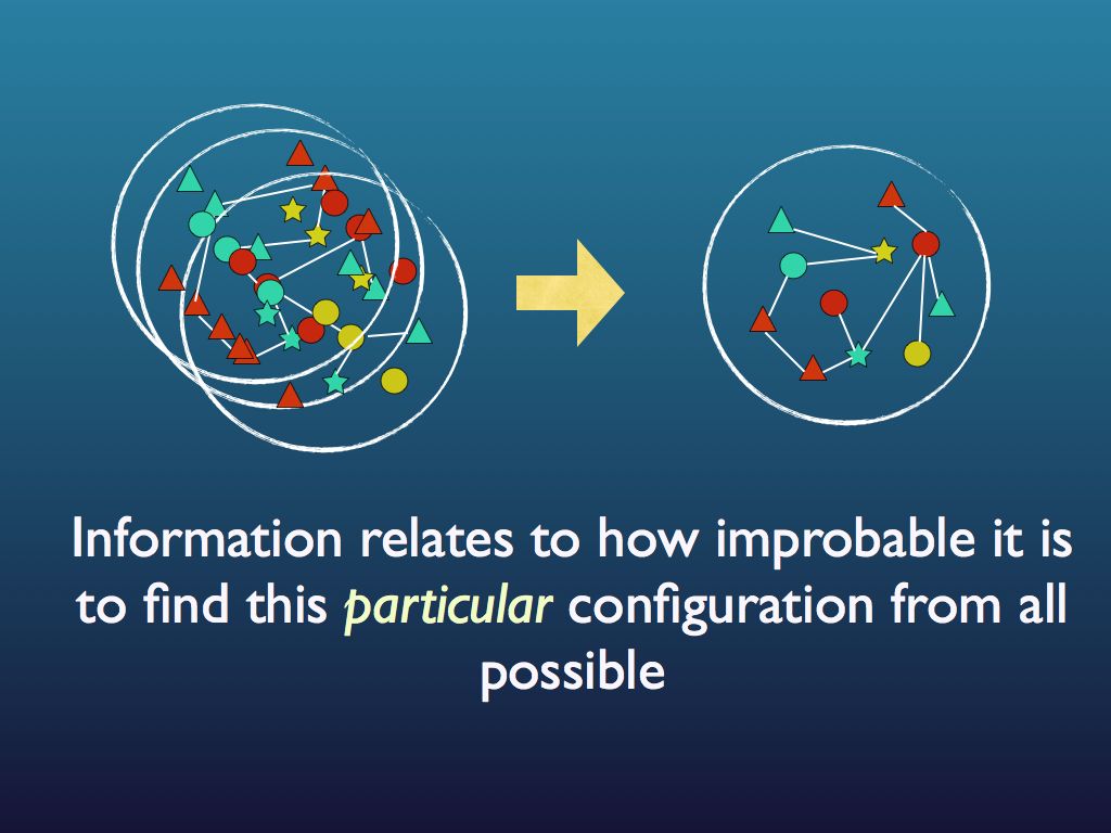
This illustrates the fact that information is a measure of how unlikely a particular signal, or configuration is to get.
Some Configurations are more likely than others
So far, we have not allowed for the fact that some configurations could be difficult (or even impossible) to achieve in practice: they may be unstable, opposed by the physics (like pushing north poles together), or they might be made easier to reach by the same physics (especially if they are energy minimising equilibria). We can take account of these natural influences by allowing the probability of each potential configuration to be biased by their physical likelihood. In effect, the physical constraints impose likelihood constraints which in turn constrain the information that can be carried by the assembly. In the extreme, imagine only one configuration is ultimately possible: for example that of a crystal lattice, which inevitably forms by energy minimisation as the assembly (e.g. of atoms) cools. Then the will be no doubt about the configuration realised, no uncertainty and no scope for differences. There would therefore be no information because there really would be only one configuration. The entropy of this constrained configuration would be at a minimum, precisely and only because of the constraint applied to the range of possible configurations. That's an extreme case, in more usual circumstances, we just face different configurations occurring with different probabilities. It is in taking account of this that the entropy measure really shows its strength, because it can represent the effect of these constraints on the realised information capacity of the ensemble, and in a most natural way.
We have already seen an example of this in the counting of lumps, where the number of configurations producing a given number of lumps depended on that number of lumps (e.g 6 configurations all produced 3 lumps). Let's continue to work with that. If we are only looking for information in the number of lumps, then there is a lot of redundancy because all 6 configurations give us the same information: 3 lumps.
Here is the table again:
number of lumps: 1 2 3 4 5
number of configurations: 1 4 6 4 1
There are a total of 2^5=16 configurations, so the proportion of the total number that are e.g. in 2 lumps is 4/16 = 1/4 and we can see the proportion for each number of lumps and understand that this is the probability of finding that number of lumps in a random assembly of the 5 blocks (e.g. 3/8 for 3 lumps and 1/16 for one lump). Clearly this lump description of the configurations conveys, and indeed embodies, less information than resolving all 16 configurations would. We can write the random likelihoods of numbers of lumps this way:
p(1) = 1/16
p(2) = 4/16
p(3) = 6/16
p(4) = 4/16
p(5) = 1/16
There are 16 configurations in total, so we need 5-bits of information to represent them all individually [ log2(16)=5]. We can also write this as log2(1/q), where q=1/16 and that is useful because 1/16 is the probability of any configuration appearing at random.
In the case of p(1) and p(5), these are as unique as the configurations themselves (only 1 configuration gives 1 or 5 lumps), so the probability of 1 or 5 lumps is also q=1/16 and therefore we need 5 bits of information to identify them. Now, take for example p(4) = 4/16. We can start with 5 bits for this too, but we do not need all 5 bits of information to represent p(4) because a lot of the information is redundant (since it distinguishes between the four configurations giving 4 lumps and we don't need that). We don't need different representations for these four configurations, so let's dump them. They represent 4 redundant configurations, so unnecessarily take up log2(4)=2 bits of information. We remove these bits from the 5 that we originally had for p(4) and get 3 bits of useful information for p(4).
We can do the same, starting with 5 bits for each number of lumps and then dumping the redundant bits to get the following:
p(1) = 5 bits
p(2) = 3 bits
p(3) = 2.42 bits (because 5-log2(6)=2.42).
p(4) = 3 bits
p(5) = 5 bits
On the face of it we have not gained much efficiency in representation here, not until we realise that the cases with higher information demands are relatively rare: p(1) is six times less common than p(6). On average, then, the amount of information needed to convey or embody this lump-code of configurations is rather less than is needed for the 'raw material' of configurations of 5 blocks. So it should be, but we want to know by how much. Well if blocks are reconfigured over and over again at random, then we can easily calculate the minimum amount of information needed to describe the process (and therefore the actual information content of the kaleidoscoping assembly of configurations). Sometimes it will be one lump that comes up and we need 5 bits, more often it will be 2 or 4 lumps, for which we only need 3 bits and so on. On average, it will be:
1 times 5 bits + 4 times 3 bits + 6 times 2.42 bits + 4 times 3 bits + 1 times 5 bits, over 16 times.
That is:
1 log2(16) + 4 log2(4/16) + 6 log2(6/16) + 4 log2(4/16) + 1 log2(16) over 16 times;
which is
1/q log2(1/q) + 4/q log2(4/q) + 6/q log2(6/q) + 4/q log2(4/q) + 1/q log2(1/q) over 1 time on average
(remember q=1/16);
which is
Sum[i=1,5] p log2(p) ( taking the definition of p from the tables above, e.g p(2)=4/16 ).
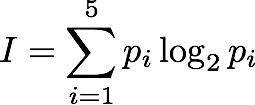
Just one problem: because logs of fractions are negative, the sum turns out to be negative and we don't really like that. Shannon multiplied the result by -1 and called it entropy.
So we now have the maximum amount of information that can be embodied in the lump code, based on assuming it was a random process - and it turns out to be exactly the same as the value given by Shannon's formula for information entropy. That's no accident.
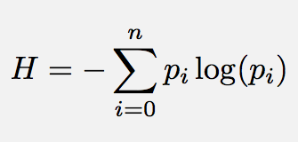
If you look at the little formula above, it is easy to see that this can be generalised to work for any assembly or configuration-generating system of any size. We first need to count the number of possible configurations and call it N (it was 5 in our previous example). Then for each of them, work out (or discover from observation) how often they are likely to happen (which might be vary rarely because of e.g. physical constraints) and attach this probability to each (p_i). Then calculate the sum of all the -(p_i log2 p_i) terms: one for each of the {i=1...N} configurations. This sum is the Information Entropy (intropy).
You will see that it does not really distinguish between information and entropy: the two seem to be synonymous. This is true, only in the restricted sense of quantifying information and of course information entropy (as opposed to the thermodynamic variety). In this sense, information does not really mean what we usually refer to in common language, where it conveys meaning as well as being quantifiable. The kind of information being added up in the Shannon formula is just the quantity of information (in bits) that a system can hold and convey - remember the fruit in the bowl that you could make secret messages with.
Earlier, I said that information was is a measure of how unlikely a particular configuration was. The more possible configurations (e.g. because more fruit in the bowl, or more kinds of fruit), the more unlikely any one of the possible configurations becomes, simply because there are more other configurations that it could have been. Now we have added the nuance that some of those configurations may have been hard to make in practice (e.g. orange balanced on a pear : physical constraints), so we don't expect them. You can see from the little calculation above, that such rare configurations require the full capacity of information of the whole assembly to represent them because there is no redundancy to describing unique events. Three fruit in a row would be common, there are lots of ways to put three in a row, so there is lots of redundancy and consequently not as much information is needed to convey this.
Now, I am sure you can work out the intropy of a traditional gambling fruit machine, but perhaps also you are getting fed up with all these probabilities.
| Why
all the probabilities? - how cell signaling really works You might wonder why we have to deal with randomness and probabilities, when really we are interested in information and the amount of it we can pack into a configuration of components. I cannot think of any explanation of entropy that does not depend on talking of dice or coin tossing or some other probabilistic process - so why? The simple answer is that Intropy was first conceived by Claude Shannon to answer the practical engineering problem of finding how much information can be transmitted over e.g. a telephone line, in the face of random noise and corrupting errors (e.g. clicks and whistles). To do this, he naturally started by describing random signals and working out what was statistically most likely to happen to them. So the simple answer is that we are borrowing a theory that was intended for a different purpose. But actually Shannon's results apply much more broadly, which is why they are so powerful. All biologists know that When DNA is transcribed, it is in principle the same as transmitting data and random mistakes can happen, so the cell faces the same sort of problem as the telephone engineer. Less well known (until you read this), biologists have a more general motivation for thinking about information in terms of probabilities: it is to do with real-life chemistry. Hormone >-- Receptor systems. Consider, for example a hormone receptor embedded in the surface of a cell. It may bind to a specific hormone such as epinephrine as the starting point for a molecular pathway inside the cell that regulates the cell's response to other hormones (via cyclic AMP) - the famous 'first and second messenger system'. This will be familiar to cellular biologists, as will the diagram showing the receptor binding to the hormone and the subsequent cascade of molecular events within the cell. What this does not convey is the fact that on the cell surface we have not one, but thousands of instances of this particular type of receptor and hormone - leading to thousands of instances of the molecular pathway to which they are connected. Real-life chemistry is not one single molecule interacting with another, it is at least thousands, often millions of such molecules interacting and they don't all do it in unison. The true picture is of a field of receptor proteins (like turnips in a field) waiting for their hormone signal molecule and at any given moment some are bound to it and others not. The cellular response at a given time depends on how many are bound at that time and this, of course, depends on the concentration of hormone. If half of the receptors are bound, then the probability that any one of them is bound equals 0.5; if all of them are, then it's 1.0. In other words, there is a relationship between the probability of any one receptor being bound and the concentration of hormone. Now, what is the probability that a particular proportion of bindings happens at any given time? You know it depends on the probability of a receptor binding and also on the concentration of hormone. We can imagine the receptors all in a row, labeled 1 if bound and zero if not. Immediately we are back with our 11001010 binary codes to represent the assembly of receptors. The cell will 'respond' to the hormone as soon as a threshold proportion of receptors are in the bound (1) state. Let's say there are 8 receptors and the threshold is 5. It doesn't matter which receptors are bound and not, just how many of them. From 00000000 to 11111111 there are 2^8 = 256 possible configurations of bound and unbound. Of these we want to know how many configurations have at least 5 1s, that is 5, 6, 7 or 8 of them. To find how many have 8 bound is easy - just one configuration can have that many. For less than 8, it is actually easier to count zeros. For 7, we can put the single zero anywhere, so there are 8 possible configurations. For 6, it's harder to work out, until we realise that finding how many ways there can be 2 zeros among 8 digits is just a combinations problem (its combinations rather than permutations because we admit all possible orderings). The answer for 6, then, is C(8,2) [using standard notation] = 8!/(2! 6!) = 7x8 / 2 = 28. For 5, we have C(8,3) = 56. Now just add these all up to get the number of at least 5 1s (3 or fewer zeros): 1 + 8 + 28 + 56 = 93. So with a response threshold of 5 bound receptors out of 8, the cell will be activated in 93/256 (about 0.36) of possible configurations. We might as well work this out for some other activation thresholds. Here is a table showing the number of combinations that will cause cell activation under different thresholds: Activation Threshold 1 2 3 4 5 6 7 8 Number of configurations 255 247 219 163 93 37 9 1 For those that want to know, the general formula for the proportion of configurations of N receptors in which at least k are bound is Pr(N,(N-k)) = 1+ Sum[i=1,(N-k)] ( C(N, i) ) / 2^N. Now let's specify the probability of any receptor being bound given a specific hormone concentration. An easy way to think of it is that if the concentration of hormone molecules is 1 in among 100 other molecules, then the probability of a hormone rather than something else bumping into the receptor site is 1/100 (i.e. 0.01). If we have 8 receptors on the cell surface, looking at this concentration, then the chance of any single one binding immediately is the chance of the first, or the second.... or the 8th. This is analogous to tossing a coin 8 times (or 8 coins simultaneously), but a coin that is weighted so that 'heads' only comes up on average 1/100 of times. We are interested in finding how likely we get e.g. at least 1 heads from the 8 tosses. Let's briefly simplify. If there were just two fair (50-50) coin tosses, the probability of at least one heads would be 0.5 (from the first toss) plus, if that had been tails (with prob.=0.5), the second toss producing heads (prob.=0.5). Note the 'if' - it tells us the second part of the sentence is conditional and we have to use a conditional probability: p(heads) on condition (given) we already had tails. The rule for combining conditional probabilities is you multiply them. So we have 0.5 from the first toss and 0.5x0.5 from the second. Either of these will do: that is we are counting the probability of either the first toss being heads, or the second (given the first was tails). The rule for combining probabilities of things where either one or the other is fine, is that we add up the probabilities. Thus we have the total probability of heads turning up at all as 0.5 + 0.5x0.5 = 0.75. If there were 8 coins, it will be 0.5 + 0.5x0.5 + 0.5x0.5x0.5... up to 8 of the 0.5s multiplied together. Notice also that for 2 coins, only 4 possible outcomes exist: HH, TT, HT, TH and only one of the 4 has no heads, so 3/4 have at least one heads: that's the 0.75 probability. So with 8 tosses, we have 2^8=256 possible outcomes (these are all the possible configurations - remember that?) so how many of them have no heads at all? The answer of course is just one: the case of 8 tails. So the probability of at least 1 heads is easy to see: it is 255/256. Notice that what we did with the maths for combining probabilities can be generalised with this formula: P = Sum[i=1,N]p^i , where p is the probability of heads, (or binding), and N is the number of tosses (or receptors). Note also that if we multiply by 2^i (which is the number of possible outcomes (or configurations of receptor binding states), we get the number of of configurations in which at least one is heads (or at least one receptor is bound). Now let's return to the receptors facing a concentration of 0.01 hormone molecules. This is represented by biased coins such that H comes up only 1/100 times on average. If there were just two receptors, the total probability of one being bound is 0.01 + (1-0.01)x0.01 which is 0.0199. Can you see why the second term is 1-0.01 here? The reason is that when considering the second toss of the biased coin, we are calculating getting a heads, on condition (given) that the first toss got tails and the probability that that happened is the probability of tails, which is 1- 0.01 (=0.99). Now, we can modify our formula calculating the number of configurations with at least one heads, to take account of this [it wasn't really wrong, but it just worked in the special case of a fair coin, where p(H)=p(T)]. The more general formula that can take any probability of heads (or binding etc.) is this: 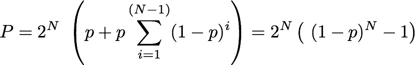 In words, this is the total number of possible configurations, times the probability that a configuration of N receptors has any that are bound, given a binding probability of p. That probability (in the big brackets) is the probability that the first one bound (the first p term) plus, if it didn't (1-p) We can now use this formula for P with N=8 and p=0.01 to find the total number of configurations in which at least one receptor is bound, when there are 8 receptors, and a hormone concentration of 1/100. I used a computer to work it out and the answer is 256x 0.0772553 = 19.777 (note the 2^N part (256) converts the probability into the number of configurations for which it is true). This might seem a bit weird because we don't have a whole number of configurations: 19.777 out of 256 possible have at least one receptor bound. Well, the reason is that we are now working with probabilities, rather than explicitly counting configurations (as we had been before). This number 19.777 is the average (expected) number of configurations with at least one receptor bound. On a different occasion, there could be more of fewer of them, but on average, this is how many to expect. The entropy of a cellular hormone detector system So what we have here, folks, is an analogue to digital converter (interface). The hormone receptor, as the first step in a 'first and second messenger system' is a piece of natural molecular-scale technology that does the same job as the A/D converter in a digital microphone. If you look closely, this sort of system can be found all over any organism (consider e.g. how your cochlea picks up sound and converts it into nerve impulses). With this in mind, we can now work out how much information a given hormone receptor array can convey to its cell. The means of quantifying it is just to find its entropy, because it is the entropy of the system that quantifies its information capacity. We use the Shannon formula (below) to do this. But first we need to specify how many states there are: that is how many conditions do we need to specify a p for in p log(p). The default position is the maximum number possible given the N receptors (this is 2^N). But, we already noticed that there is no meaningful difference between e.g. 1001 and 1100, because all that matters is only how many receptors are bound - their individual identity is of no concern. We really want to define a state as a number of receptors bound, rather than a configuration. With N receptors, obviously you could have any number from zero to N that are bound and each of those N+1 numbers is a state for which we need the p. But we also know that doing this, most of the states are fulfilled by several configurations (e.g. 1001 and 1100 are two different configurations that belong to the state of having two receptors bound). To account for these, we just count up the number of configurations which have exactly the same number of bound receptors (in that example 2 of them). We have done something very similar above - we used combinations. The number of configurations of an N-receptor array that has k bound is C(N,k). Working the probabilities out is easy (assuming the receptors don't affect each other). To keep it general, let's write the answers in terms of the binding probability (which to avoid confusion of p's, will be given the symbol b here, so the probability of a single receptor being unbound is (1-b)). The probabilities of each of the 6 possible states are in the following table for a 5 receptor array: Number bound: 0 1 2 3 4 5 probability p: (1-b)^5 b(1-b)^4 b^2 (1-b)^3 b^3 (1-b)^2 b^4 (1-b) b^5 number of ways: C(5,0) C(5,1) C(5,2) C(5,3) C(5,4) C(5,5) number of ways: 1 5 10 10 5 1 In the 3rd row of the table I put the combinations formula for how many configurations are in each of the states and I worked out the numerical value of this in the 4th row. Now, in the Shannon formula, the p we want is the probability (second row) times the number of ways that can happen (4th row). I'm sure you can see the pattern in that and can generalise to N receptors. The kth state, with k receptors out of N bound, has p= (1-b)^(N-k) b^k and it can happen in C(N,k) ways. We can add these up for k=1 to N in the Shannon formula (that's what it tells us to do). Just as a simple check if there are 2 receptors, then the entropy of the A/D converter is H = - [ 1(1-b)^2 log2 ( 1(1-b)^2) + 2 b(1-b) log2 (2 b(1-b)) + 1 b^2 log2 (1 b^2), in which the first term is p of state 00, the third term is p of 11 and the second term is p of 01 or 10 (there are two of these single-bound states so we multiplied the p by 2 (as C(2,1) tells us). Just so you can see it, here is the formula for each of the p terms in the Shannon formula: 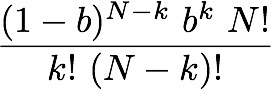
There is one of these for each of the p log2p terms in the Shannon formula, where the index i is what we have as k in this p-term formula (remember k is the number of bound receptors, running from zero to N of them. Using the Shannon formula (which you see below), just adding up the p-terms from i=k=1 to N, we can find the entropy of receptor arrays. For a hormone concentration of 0.01, (approximate) H is calculated for a few array sizes below: N in the array: 1 2 5 8 64 H(0.01): 0.081 0.142 0.289 0.409 1.521 and for comparison, here are the entropies with concentration of 0.5 (simulating the fair coin toss): H(0.5): 1 1.5 2.198 2.544 4.047 The entropies when concentration is 0.01 are much lower than when it is such that there is a 50/50 chance of a single receptor binding. This is because there is not much information conveyed by a 'signal' from the receptor array that says "no hormones found here". In simple terms, the response of the receptors (binding) is so insensitive that the cell would never be 'surprised' to find that they were not signaling a presence of the hormone: almost all the time they would not be. If the chance of binding was 50/50, though, even with just one receptor, the cell has no idea whether there is hormone or not (it cannot anticipate or guess the binding state of the receptor) until it has received the signal. In this case it is gaining the maximum possible amount of information from its one receptor and the entropy is as big as it can be for a single receptor: it is 1. If you then look at the 2-receptor case, again with 50/50 chance of binding, we have the same situation as we had in tossing 2 fair coins. The chance of a binding is 3 in 4 when the hormone is present, so the entropy is that for a probability of 3/4, which turns out to be 1.5. If you are still uncertain about that, please read Sriram Vajapeyam's article (see links at the bottom of this page) to get it from a slightly different angle. Let me leave this box with the Shannon formula I used for working out the entropy of receptor arrays: I copied this out of Mathematica ©, which is what I used to perform the calculations. 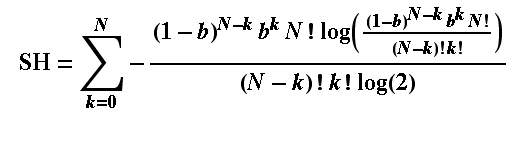 You can try this yourself: put the formula into a computer and work out the Shannon entropy of any size of hormone receptor array as a function of the hormone binding probability (our surrogate for hormone concentration (just note - the log(2) is a natural log used to convert everything to log base 2 units). |
The Shannon Formula
Shannon’s information entropy (intropy) quantifies the average number of bits needed to store (embody) or communicate a message. From the 20 questions analogy above, we saw that at minimum one needed to ask log2(n) binary questions in order to fully specify (know or apprehend) a piece of information that is the size of an n-bit binary string. For communications engineers, Shannon’s entropy determines that one cannot store (and therefore communicate) a piece of information of length n symbols in less than log2(n) bits. In this sense, Shannon’s entropy determines the lower limit for compressing a message, and that is close to its original purpose. For biologists, we see that (as illustrated in the green box above), life's information processes can generally be reinterpreted in terms of binary strings of activated / not activated molecules, or pathways, and these are naturally affected by random chance, simply because all of life's chemistry is really a matter of molecules randomly bouncing about in a jiggling aqueous solution (see the beautiful illustrations by David Godsell to get a good impression of that).
Note the log here is in base 2 (for information units of bits), but it does not have to be in log base 2. For example if we were coding the information in DNA or RNA, then we would have 4 different symbols and the code would therefore not be binary, but quaternary and we would best use log base 4.
Information as the change of Intropy under constraint
Lastly, let us return briefly to the idea that information is a measure of the 'surprise' of a message (so often stated by information theory experts). What they mean is that the less likely an observation is, the more information is conveyed by observing it. That does not mean it is more powerful or meaningful information because we are just quantifying bits here, not meaning. All it amounts to, is saying that: relatively rare things need more information to express them than relatively common things. I emphasise the word relatively there because it reveals an important hidden assumption. The idea is that there is a finite set of configurations or 'messages', so a few common ones probably make up a large part of the total, leaving the rest to very many different but rare ones. An often quoted example of this sort of uneven distribution is Zipf's law for word frequencies in English language text (and Zipf found that log(frequency of use)=-log(rank) in James Joyce's Ulysses). A rare word is, in a statistical sense, a surprising word, but there are quite a lot of them, whereas there are only few common words (because if there were a lot of these as well then they could not be common because our finite number of configurations would be over filled - we would run out of possible 'messages' if there were a lot of different common words. No, we only have room for a lot of words that are rare. Well, if there are a lot of them, then obviously we need a lot of configurations to represent them all (one for each). So, in terms of the total amount of information (configuration space) used up by these rare words, it is more than the amount used up by the few common words.
When someone says that a system has lost entropy - is in a lower entropy state, or (horror! has become less disorganised), what (they should) mean is that it has been constrained by something to occupy a reduced configuration space - i.e. a condition has been applied that reduces the number of available possible configurations. On the roulette wheel we may say 'black only' - halving the configuration space and by doing so, reducing the entropy of the game and by that, conveying information. In this sense (only) information is the converse of intropy. This reduction of intropy by constraint is so useful, though, that information theorists often fall into referring to the constrained system as a (relatively) low entropy system. This is where we get the unfortunate misconception about organised systems being of low entropy.
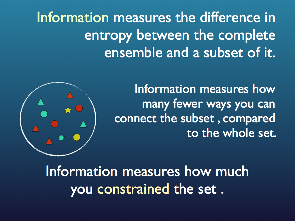
Entropy is typically measured relative to the maximum entropy system, which is of course the complete set of elements or configurations. As the elements are put into a particular (perhaps functional) order, the whole system does not change entropy, but the resulting constrained sub-set of configurations that make up the 'ordering' does have a lower entropy relative to the full set, because there are fewer options for configuring it - obviously because it has just been constrained. Less is more!
The link between thermodynamic entropy and information in living systems.
Stuart Kaufmann defines life in terms of the minimum (complexity) living thing, which he calls an ‘autonomous agent’ and it has the following attributes: it is an auto-catalytic system contained within a boundary (a membrane) and it is capable of completing at least one thermodynamic work cycle. This recognises that whatever living is, it must use energy to perform work: to build itself, to differentiate itself from the wider environment, to move, replicate and repair itself. All these features of the living require energy to be ‘degraded’ (for example from light into heat) in order to 'upgrade' the living form. What is meant by degrade and upgrade here is the amount of entropy: the higher the entropy, the lower the 'grade'. In effect high grade energy is more constrained than low grade: it has fewer degrees of freedom for its action. As we saw above, that means there are fewer ways it can be configured (for example, fewer ways molecules can move about in a gas). This matters because, by the Second Law of thermodynamics, the total number of ways to configure a system can only increase (entropy always increases). Because life always has to reduce its entropy (constantly creating and maintaining its specific structure) it has to get something else to increase in entropy instead - as a counter balance. It does this by coupling its structure to passing energy; as the energy flows past, life passes its 'excess' entropy onto the energy. The requirement for a thermodynamic work-cycle is another way of saying that a living organism is a kind of engine. That is a system which 'pumps entropy' into energy to provide a source of work. In effect, all living systems are engines that transfer entropy from an organism into the environment (especially by degrading energy). This might leave us puzzled, since entropy was defined at the beginning as a measure of the number of ways a system can be configured, so talk of it being 'pumped' seems to make no sense. It is figurative language that more precisely means that an engine is a system for changing the number of ways that passing energy can be configured.
In fact, thermodynamic entropy is defined by the Second Law of thermodynamics, in which it has the (classical) simple meaning of heat divided by absolute temperature: S := W / ºK. Probability comes into this because heat is in fact the sum total of the individual kinetic energies of atoms and molecules and this can be calculated using statistical mechanics, which in turn uses probability calculations. Crucially, the greater the heat, the more ways there are for a set of particles (be they atoms or molecules) to make up the total energy - this number of ways is termed the ‘multiplicity of the system’. For example, if there were just three particles and the total energy was 5 (tiny units), then, assuming only integers values, there would be 5 ways to make up this total using integer energies. If it were 10 units, there would be 14 ways. In reality it is not that simple: energies are not integers and the number of particles is, in practice, enormous (Avagadro’s number is about 6x10^23), so the multiplicity is expressed via a probability distribution. The probability distribution expresses the likelihood of total energies, given the number of ways you could make up each total energy from the individual particle speeds (the basis of their kinetic energies). For an ideal gas, the particular distribution is (fittingly) the Maxwell* distribution and it depends on the square root of temperature. To find a more thorough explanation of all this, we recommend visiting here.
* Named after one of the ‘fathers’ of statistical mechanics (and much besides): James Clerk Maxwell.
Historically, The two concepts bearing the same name ‘entropy’ are first thermodynamic entropy and second information entropy. The confusion arises because, in a development that has become infamous in the history of physics, Claude Shannon, having derived a term relevant to information transmission, was advised to name it after the earlier defined entropy of thermodynamics because it has the same mathematical form. Some have argued that the two have nothing at all to do with each other and that the simile is only a coincidence. This denies the fact that both can be derived from an argument using the frequencies of number combinations to find the probability of different microstates (see below). There is then, a probability theory root to both, but they still do refer to very different things in the end.
The statistical principles underlying thermodynamic entropy are the same statistical principles as underly information entropy, but that is the only connection between them.
Life as a persistent branch-system.
Entropy is defined by the Second Law of thermodynamics. Boltzmann derived the second law from statistical mechanics and ever since, this has been widely taken to mean that closed** systems tend towards their entropy maximum, simply through probability. However, this is not true; in fact the chance of entropy increase is matched by that of decrease as closed systems, over the long run are expected to fluctuate from the maximum entropy, taking random dips from it with a frequency inversely related to their magnitude. This is because all the microscopic processes of thermodynamics (molecular movements etc.) are strictly reversible, so since entropy is entirely and only dependent on them, there is no reason why entropy should always increase. The understandable mistake comes from thinking of common applications where entropy starts low and the time-course of the system’s dynamics are thought of over a relatively short span (for example a kettle cooling). It turns out, though, that these familiar small systems are best thought of as sub-systems of a larger system which is randomly dipping from maximum entropy equilibrium. Paul Davies reminds us of a footprint in the sand on a beach: it is clearly a local drop in entropy because it forms a distinct and improbable pattern that is out of equilibrium with the flat surface around it. We intuitively know that it will dissipate as its entropy rises. However, it is wrong to assume that this is because it is part of the whole beach for which entropy is always rising to a maximum. In fact the footprint was made by a process beyond the beach which caused a small part of the beach to branch-off temporarily into a separate system. Branch systems form by external influences and if left alone, they dissipate to merge back into their parent system over time. The forming of a lower entropy branch system this way, involves a more than counter-balancing increase in entropy globally. So, what of life? We can see this as a branch system in the universe, but one that is continually replenishing its low entropy by pumping out entropy into the rest of the universe, via degrading energy. Life is a continually renewing branch process.
** In thermodynamics, closed refers to a system surrounded by a boundary across which energy, in the form of work or heat, but not matter, may pass or be exchanged with its surroundings.
Work and Life
Life is only possible if it can do work (in the technical sense used in physics). The textbook definition of work in this technical sense means the result of a force acting over a distance in a particular direction and you might ask what that has to do with living. The answer is that in thermodynamic equilibrium, matter consists of a lot of particles moving in random directions, hence with random momentum and this results in forces (for example gas pressure) that have no coherent pattern to them, so that on average (and we are averaging over huge numbers of particles) forces balance, so there is no net movement. This lack of net movement is a result of incoherence, of randomness and therefore of lack of pattern and therefore lack of embodied information. There is kinetic energy in all the incoherent movement, but in this random configuration, it cannot yield any work. For that we need some coherence to the momentum of the particles and this is achieved by limiting their scope, that is by constraining them (for example with a chamber and piston), which of course is equivalent to reducing the entropy of the system. Work is possible when there is a net direction to forces and this necessarily implies some organised pattern to the movements. Organised pattern, in turn, implies information. Once energy is organised into some information instantiating pattern, that pattern-information can be transferred to another component of the system. A thermodynamic work cycle (referring again to Stuart Kaufmann’s observation) is a process of extracting work from organised energy by transferring the information of organisation into another form, or part of the system. So, for example, constructing a protein molecule is an act of organising matter and to do it, life must sequester that organisation from energy. It is in this sense that catabolism (making body parts like protein molecules) uses energy. The energy is not used up (the First Law of Thermodynamics ensures that energy is never created nor destroyed); rather energy is disorganised, taking the information out of it to use in the catabolic process. The energy of photosynthetically active radiation (e.g. red and blue light) is more organised that that of heat radiation, so in transforming sunlight into warmth, plant leaves are supplying the necessary ‘organisation’ for constructing plant body parts. This ‘organisation’ is the information embodied in organic molecules: first in sugar (as a sort of currency), which is then transferred into a wide variety of molecules and structures built from them. Whenever energy is converted from a ‘high grade’ such as light to a ‘low grade’ such as heat, work can be extracted and used to construct something or perform a coherent action. Since living consists of a set of coherent and highly organised chemical reactions, many of which are also catabolic, there is plenty of need for work. Life would not exist without it.
Some Links on Entropy
In my experience, properly appreciating entropy only happens gradually as one reads lots of different accounts and thinks about them. For this reason, I recommend getting to know a few more, starting with the list below.
Shannon entropy explained by picking balls from buckets this is a different explanation of entropy that seems quite complementary.
Sriram Vajapeyam has put this really excellent explanation of entropy calculation on ArXiv (the physics publication archive site) https://arxiv.org/pdf/1405.2061.pdf - Highly recommended!
Here is one of the nicest you-tube explanations I have found (be aware that some are just wrong).
Stack exchange Answers - stack exchange people give some more rigorous and mathematical explanations - a nice adjunct to what is here.
The Journal 'Entropy' : yes, there is a whole scientific journal devoted to entropy and what you can do with it.
Here is the start of a very nice series of you-tube talks on Information Theory (as a more general concept, including the development of writing) .
Better Explained has a number of basic and intermediate maths explanations that I recommend. The link here is to their explanation of permutations and combinations, which this article uses.
Hyperphisics gives a nice account of entropy, focusing on the thermodynamic variety - you cannot go wrong with them. http://hyperphysics.phy-astr.gsu.edu/hbase/Therm/entrop.html